Author Archives: Shanoj

Unknown's avatar

About Shanoj

Author : Shanoj is a Data engineer and solutions architect passionate about delivering business value and actionable insights through well-architected data products. He holds several certifications on AWS, Oracle, Apache, Google Cloud, Docker, Linux and focuses on data engineering and analysis using SQL, Python, BigData, RDBMS, Apache Spark, among other technologies. He has 17+ years of history working with various technologies in the Retail and BFS domains.

Data Modeling 101: Modern Data Stack

What is Data Modeling?

Data modeling is the foundational process of creating a structured representation of data stored in a database. This representation, a data model, serves as a conceptual blueprint for data objects, their relationships, and the governing rules that ensure data integrity and consistency. Data modeling helps us define how data is organized, connected, and utilized within a database or data management system.

Common Data Modeling Approaches:

Normalized Modeling:

The normalized modeling approach, popularized by Bill Inmon, is focused on maintaining data integrity by eliminating redundancy. It involves creating a data warehouse that closely mirrors the structure of the source systems. While this approach ensures a single source of truth, it can lead to complex join operations and may not be ideal for modern column-based data warehouses.

Denormalized Modeling (Dimensional Modeling):

Ralph Kimballโ€™s denormalized modeling, dimensional modeling, emphasizes simplicity and efficiency. It utilizes a star schema structure, which reduces the need for complex joins. Denormalized modeling is designed around business functions, making it well-suited for analytical reporting. It strikes a balance between data redundancy and query performance.

Data Vault Modeling:

The Data Vault modeling approach is complex and organized, dividing data into hubs, links, and satellites. It focuses on preserving raw data without compromising future transformations. While it is excellent for data storage and organization, a presentation layer is often required for analytical reporting, making it a comprehensive but intricate approach.

One Big Table (OBT) Modeling:

The OBT modeling approach takes advantage of modern storage and computational capabilities. It involves creating wide denormalized tables, minimizing the need for intermediate transformations. While this approach simplifies data modeling, it can increase computational costs and data redundancy, particularly as the organization scales.

Why is Data Modeling Important?

Now that we understand what data modeling entails, letโ€™s explore why it holds such significance in data management and analytics.

Visual Representation and Rule Enforcement:

Data modeling provides a visual representation of data structures, making it easier for data professionals to understand and work with complex datasets. It also plays a crucial role in enforcing business rules, regulatory compliance, and government policies governing data usage. By translating these rules into the data model, organizations ensure that data is handled according to legal and operational standards.

Consistency and Quality Assurance:

Data models serve as a framework for maintaining consistency across various aspects of data management, such as naming conventions, default values, semantics, and security measures. This consistency is essential to ensure data quality and accuracy. A well-designed data model acts as a guardian, preventing inconsistencies and errors arising from ad-hoc data handling.

Facilitating Data Integration:

Organizations often deal with data from multiple sources in today’s data-rich landscape. Data modeling is pivotal in designing structures that enable seamless data integration. Whether youโ€™re working with Power BI, other data visualization tools, or databases, data modeling ensures that data from different entities can be effectively combined and analyzed.

Things to Consider:

Organizational and Mental Clarity:

Regardless of the chosen data modeling approach, organizational clarity and mental clarity should remain paramount. A structured data modeling strategy provides a foundation for managing diverse data sources effectively and maintaining consistency throughout the data pipeline.

Embracing New Technologies:

Modern data technologies offer advanced storage and processing capabilities. Organizations should consider hybrid approaches that combine the best features of different data modeling methods to leverage the benefits of both simplicity and efficiency.

Supporting Data Consumers:

Data modeling should not cater solely to individual users or reporting tools. Consider a robust data mart layer to support various data consumption scenarios, ensuring that data remains accessible and usable by various stakeholders.

๐ŸŒŸ Enjoying my content? ๐Ÿ™ Follow me here: Shanoj Kumar V

Stackademic

Thank you for reading until the end. Before you go:

  • Please consider clapping and following the writer! ๐Ÿ‘
  • Follow us on Twitter(X), LinkedIn, and YouTube.
  • Visit Stackademic.com to find out more about how we are democratizing free programming education around the world.

Apache Flink 101: Checkpointing

Checkpointing in Apache Flink is the process of saving the current state of a streaming application to a long-term storage system such as HDFS, S3, or a distributed file system on a regular basis. This enables the system to recover from failures by replaying a consistent checkpoint state.

The following are the primary use cases for checkpointing:

  • Stateful Stream Processing: The checkpointing feature of Apache Flink is especially useful for stateful stream processing applications. For example, a real-time fraud detection system that saves the state of a userโ€™s transactions can use checkpointing to save the state regularly and recover it in the event of a failure.
  • Continuous Processing: Checkpointing can also implement continuous data stream processing. If the application is checkpointed at regular intervals, it can be resumed from the last checkpoint in case of a failure, ensuring no data is lost.
  • Event-Driven Applications: It is critical in event-driven architectures to ensure that events are processed in the correct order. Checkpointing can be used to ensure that the applicationโ€™s state is preserved.
  • Machine Learning and Data Analytics: Checkpointing is also useful in machine learning and data analytics applications where the state of the application needs to be saved periodically to allow for training models or analyzing data.
  • Rolling Upgrades: Checkpointing can be used to implement rolling upgrades of Flink applications. Checkpointing the application’s state before upgrading can be resumed from the last checkpoint after the upgrade, minimizing downtime.

Checkpointing can be enabled in a PyFlink application as follows:

from pyflink.datastream import StreamExecutionEnvironment
# create a StreamExecutionEnvironment
env = StreamExecutionEnvironment.get_execution_environment()
# enable checkpointing
env.enable_checkpointing(interval=1000, checkpoint_directory="hdfs://checkpoints")

In the preceding example, we enable checkpointing with a 1000-millisecond interval, meaning the applicationโ€™s state will be checkpointed every 1000 milliseconds. The data from the checkpoints will be saved in the โ€œhdfs:/checkpointsโ€ directory.

When checkpointing fails, specify the number of retries and the time between retries.

# enable checkpointing with retries
env.enable_checkpointing(interval=1000, checkpoint_directory="hdfs://checkpoints",
max_concurrent_checkpoints=1,
min_pause_between_checkpoints=5000,
max_failures_before_checkpointing_aborts=3)

In this example, the max concurrent checkpoints parameter is set to 1, implying that only one checkpoint can be active at any given time. The minimum pause between checkpoints setting is set to 5000 milliseconds, meaning there must be a 5000-millisecond pause between two consecutive checkpoints. The value of max failures before checkpointing aborts is set to 3, meaning the application will be terminated if three consecutive checkpoint attempts fail.

Before enabling checkpointing in the application, you must configure the storage system and the directory you want to use for checkpointing.

Stackademic

Thank you for reading until the end. Before you go:

  • Please consider clapping and following the writer! ๐Ÿ‘
  • Follow us on Twitter(X), LinkedIn, and YouTube.
  • Visit Stackademic.com to find out more about how we are democratizing free programming education around the world.

System Design 101: Adapting & Evolving Design Patterns in Software Development

Think of ๐๐ž๐ฌ๐ข๐ ๐ง ๐ฉ๐š๐ญ๐ญ๐ž๐ซ๐ง๐ฌ as solutions to recurring problems. ๐‘ป๐’‰๐’†๐’šโ€™๐’“๐’† ๐’๐’Š๐’Œ๐’† ๐’•๐’Š๐’Ž๐’†-๐’•๐’†๐’”๐’•๐’†๐’… ๐’“๐’†๐’„๐’Š๐’‘๐’†๐’” ๐’‡๐’๐’“ ๐’„๐’๐’Ž๐’Ž๐’๐’ ๐’Š๐’”๐’”๐’–๐’†๐’” ๐’Š๐’ ๐’”๐’๐’‡๐’•๐’˜๐’‚๐’“๐’† ๐’…๐’†๐’—๐’†๐’๐’๐’‘๐’Ž๐’†๐’๐’•. But what if the problem youโ€™re dealing with isnโ€™t the same as the one a particular pattern addresses? Hereโ€™s the cool part: you can often adapt existing patterns. Itโ€™s like ๐ญ๐ฐ๐ž๐š๐ค๐ข๐ง๐  a recipe to suit your taste.

However, thereโ€™s a catch. When implementing a pattern, you should always consider โ€˜๐ž๐ฑ๐ญ๐ž๐ง๐ฌ๐ข๐›๐ข๐ฅ๐ข๐ญ๐ฒโ€™. This means building in a bit of ๐Ÿ๐ฅ๐ž๐ฑ๐ข๐›๐ข๐ฅ๐ข๐ญ๐ฒ. Think of it as future-proofing. Youโ€™re saying, โ€˜Hey, this solution might need to change a little down the road when new ingredients become available.โ€™

But what if the problem undergoes a ๐ฆ๐š๐ฃ๐จ๐ซ ๐ญ๐ซ๐š๐ง๐ฌ๐Ÿ๐จ๐ซ๐ฆ๐š๐ญ๐ข๐จ๐ง? Imagine your favourite recipe changes from baking a cake to grilling a steak. Thatโ€™s when you realize the old recipe wonโ€™t work anymore. Itโ€™s time to introduce a new patternโ€Šโ€”โ€Ša new recipe perfect for the ๐ซ๐ž๐ฏ๐š๐ฆ๐ฉ๐ž๐ ๐ฉ๐ซ๐จ๐›๐ฅ๐ž๐ฆ.

In a nutshell, updating a design pattern depends on how the problem it tackles changes. If itโ€™s just a ๐ฆ๐ข๐ง๐จ๐ซ ๐ญ๐ฐ๐ž๐š๐ค, you can often tweak the pattern. But if the problem takes an entirely ๐๐ข๐Ÿ๐Ÿ๐ž๐ซ๐ž๐ง๐ญ ๐๐ข๐ซ๐ž๐œ๐ญ๐ข๐จ๐ง, itโ€™s time to welcome a new pattern into the kitchen. The key is to keep your solutions ๐ž๐Ÿ๐Ÿ๐ž๐œ๐ญ๐ข๐ฏ๐ž ๐š๐ง๐ ๐ฎ๐ฉ-๐ญ๐จ-๐๐š๐ญ๐ž as the world evolves.

Apache Spark 101:Schema Enforcement vs. Schema Inference

When working with data in Apache Spark, one of the critical decisions youโ€™ll face is how to handle data schemas. Two primary approaches come into play: Schema Enforcement and Schema Inference. Letโ€™s explore these approaches with examples and a visual flowchart.

Understanding Schema in Apacheย Spark

In Apache Spark, a schema defines the structure of your data, specifying the data types for each field in a dataset. Proper schema management is crucial for data quality and efficient processing.

Schema Enforcement: A Preferred Approach

Schema Enforcement involves explicitly defining a schema for your data before processing it. Hereโ€™s why itโ€™s often the preferred choice:

  1. Ensures Data Quality: Enforcing a schema reduces the risk of incorrect schema inference. It acts as a gatekeeper, rejecting data that doesnโ€™t match the defined structure.

For example, schema inference becomes necessary if we use strings as the data input. Let me explain further. For instance, a date might be inferred as a string, and Spark has to scan the data to determine the data types, which can be time-consuming.

2. Performance Optimization: Spark can optimize operations when it knows the schema in advance. This results in faster query performance and more efficient resource usage.

3. Predictable Processing: With a predefined schema, you have predictable data structures and types, making collaboration among teams more straightforward.

Schema Inference: Challenges toย Consider

Schema Inference, while flexible, presents challenges:

1. Potential for Incorrect Schemas: Schema inference could lead to incorrect schema detection, causing data interpretation issues.

2. Resource Intensive: Inferring the schema requires scanning the data, which can be time-consuming and resource-intensive, affecting system performance.

Sampling Ratio: Aย Solution

To mitigate the performance impact of schema inference, you can use a sampling ratio. Instead of scanning the entire dataset, you infer the schema based on a provided ratio. This helps strike a balance between flexibility and performance.

Example: In the case of schema sampling, instead of scanning the complete dataset, you can specify a sampling ratio (e.g., 10%) to infer the schema. This means Spark will analyze only a fraction of the data to determine the schema, reducing the computational overhead.

Two Ways to Enforceย Schema

1. Schema Option: You can enforce a schema using Sparkโ€™s `schema` option, where you explicitly define the schema in your code.

from pyspark.sql.types import StructType, StructField, StringType, IntegerType

schema = StructType([
StructField("Name", StringType(), nullable=False),
StructField("Age", IntegerType(), nullable=False),
StructField("Email", StringType(), nullable=True)
])

2. Schema DDL: Alternatively, you can enforce the schema using Data Definition Language (DDL) statements when reading data:

df = spark.read.option("header", "true").option("inferSchema", "false").schema(schema).csv("customer_data.csv")

When working with data in Apache Spark, choosing between Schema Enforcement and Schema Inference is critical. Schema Enforcement is often preferred for data quality and performance reasons. However, you can use schema inference with a sampling ratio to strike a balance. Remember that the choice between schema enforcement and inference depends on your data characteristics and processing needs. In many cases, enforcing the schema is the way to go for robust and efficient data pipelines.

๐ŸŒŸ Enjoying my content? ๐Ÿ™ Follow me here: Shanoj Kumar V

Stackademic

Thank you for reading until the end. Before you go:

  • Please consider clapping and following the writer! ๐Ÿ‘
  • Follow us on Twitter(X), LinkedIn, and YouTube.
  • Visit Stackademic.com to find out more about how we are democratizing free programming education around the world.

Enterprise Software Development 101: Navigating the Basics

Enterprise software development is a dynamic and intricate field at the heart of modern business operations. This comprehensive guide explores the various aspects of enterprise software development, offering insights into how development teams collaborate, code, integrate, build, test, and deploy applications. Whether youโ€™re an experienced developer or new to this domain, understanding the nuances of enterprise software development is crucial for achieving success.

1. The Team Structure

  • Team Composition: A typical development team comprises developers, a Scrum Master (if using Agile methodology), a project manager, software architects, and often, designers or UX/UI experts.
  • Software Architect Role: Software architects are crucial in designing the softwareโ€™s high-level structure, ensuring scalability and adherence to best practices.
  • Client Engagement: The client is the vital link between end-users and developers, pivotal in defining project requirements.
  • Scaling Up: Larger projects may involve intricate team structures with multiple teams focusing on different software aspects, while core principles of collaboration, communication, and goal alignment remain steadfast.

2. Defining the Scope

  • Project Inception: Every enterprise software development project begins with defining the scope.
  • Clientโ€™s Vision: The client, often the product owner, communicates their vision and requirements, initiating the process of understanding what needs to be built and how it serves end-users.
  • Clear Communication: At this stage, clear communication and documentation are indispensable to prevent misunderstandings and ensure precise alignment with project objectives.

3. Feature Development Workflow

  • Feature Implementation: Developers implement features and functionalities outlined in the project scope.
  • Efficient Development: Teams frequently adopt a feature branch workflow, where each feature or task is assigned to a team of developers who work collaboratively on feature branches derived from the main codebase.
  • Code Review: Completing a feature triggers a pull request and code review, maintaining code quality, functionality, and adherence to coding standards.

4. Continuous Integration and Deployment

  • Modern Core: The heart of contemporary software development lies in continuous integration and deployment (CI/CD).
  • Seamless Integration: Developers merge feature branches into a development or main branch, initiating automated CI/CD pipelines that build, test, and deploy code to various environments.
  • Automation Benefits: Automation is pivotal in the deployment process to minimize human errors and ensure consistency across diverse environments.

5. Environment Management

  • Testing Grounds: Enterprise software often necessitates diverse testing and validation environments resembling the production environment.
  • Infrastructure as Code: Teams leverage tools like Terraform or AWS CloudFormation for infrastructure as code (IaC) to maintain consistency across environments.

6. Testing and Quality Assurance

  • Critical Testing: Testing is a critical phase in enterprise software development, encompassing unit tests, integration tests, end-to-end tests, performance tests, security tests, and user acceptance testing (UAT).
  • Robust Product: These tests ensure the delivery of a robust and reliable product.

7. Staging and User Feedback

  • Final Validation: A staging environment serves as a final validation platform before deploying new features.
  • User Engagement: Clients and end-users actively engage with the software, providing valuable feedback.

8. Release Management

  • Strategic Rollout: When stakeholders are content, a release is planned.
  • Feature Control: Feature flags or toggles enable controlled rollouts and easy rollbacks if issues arise.

9. Scaling and High Availability

  • Scalability Focus: Enterprise software often caters to large user bases and high traffic.
  • Deployment Strategies: Deployments in multiple regions, load balancing, and redundancy ensure scalability and high availability.

10. Bug Tracking and Maintenance

  • Ongoing Vigilance: Even after a successful release, software necessitates ongoing maintenance.
  • Issue Resolution: Bug tracking systems identify and address issues promptly as new features and improvements continue to evolve.

๐ŸŒŸ Enjoying my content? ๐Ÿ™ Follow me here: Shanoj Kumar V

Stackademic

Thank you for reading until the end. Before you go:

  • Please consider clapping and following the writer! ๐Ÿ‘
  • Follow us on Twitter(X), LinkedIn, and YouTube.
  • Visit Stackademic.com to find out more about how we are democratizing free programming education around the world.

Apache Spark 101: Shuffling, Transformations, & Optimizations

Shuffling is a fundamental concept in distributed data processing frameworks like Apache Spark. Shuffling is the process of redistributing or reorganizing data across the partitions of a distributed dataset.

Hereโ€™s a more detailed breakdown:

Why it Happens: As you process data in a distributed system, certain operations necessitate a different data grouping. For instance, when dealing with a key-value dataset and the need arises to group all values by their respective keys, ensuring that all values for a given key end up on the same partition is imperative.

How it Works: To achieve this grouping, data from one partition might need to be moved to another partition, potentially residing on a different machine within the cluster. This movement and reorganization of data are collectively termed shuffling.

Performance Impact: Shuffling can be resource-intensive regarding both time and network utilization. Transferring and reorganising data across the network can considerably slow down processing, especially with large datasets.

Example: Consider a simple case where you have a dataset with four partitions:

Partition 1: [(1, "a"), (2, "b")] 
Partition 2: [(3, "c"), (2, "d")]
Partition 3: [(1, "e"), (4, "f")]
Partition 4: [(3, "g")]

If your objective is to group this data by key, youโ€™d need to rearrange it so that all the values for each key are co-located on the same partition:

Partition 1: [(1, "a"), (1, "e")] 
Partition 2: [(2, "b"), (2, "d")]
Partition 3: [(3, "c"), (3, "g")]
Partition 4: [(4, "f")]

Notice how values have been shifted from one partition to another? This is shuffling in action!

Now, letโ€™s understand Narrow vs. Wide Transformations:

Letโ€™s break down what narrow and wide transformations mean:

Narrow Transformations:

Definition: Narrow transformations imply that each input partition contributes to only one output partition without any data shuffling between partitions.

Examples: Operations like map(), filter(), and union() are considered narrow transformations.

Dependency: The dependencies between partitions are narrow, indicating that a child partition depends on data from only a single parent partition.

Visualization: Regarding lineage visualization (a graph depicting dependencies between RDDs), narrow transformations exhibit a one-to-one relationship between input and output partitions.

Wide Transformations:

Definition: Wide transformations, on the other hand, entail each input partition potentially contributing to multiple output partitions. This typically involves shuffling data between partitions to ensure that records with the same key end up on the same partition.

Examples: Operations like groupByKey(), reduceByKey(), and join() fall into the category of wide transformations.

Dependency: Dependencies are wide, as a child partition might depend on data from multiple parent partitions.

Visualization: In the lineage graph, wide transformations display an input partition contributing to multiple output partitions.

Understanding the distinction between narrow and wide transformations is crucial due to its performance implications. Because of their involvement in shuffling data across the network, wide transformations can be significantly more resource-intensive in terms of time and computing resources than narrow transformations.

In the case of groupByKey(), since itโ€™s a wide transformation, it necessitates a shuffle to ensure that all values for a given key end up on the same partition. This shuffle can be costly, especially when dealing with a large dataset.

How groupByKey() Works:

Shuffling: This is the most computationally intensive step. All pairs with the same key are relocated to the same worker node, whereas pairs with different keys may end up on different nodes.

Grouping: On each worker node, the values for each key are consolidated together.

Simple Steps:

  1. Identify pairs with the same key.
  2. Gather all those pairs together.
  3. Group the values of those pairs under the common key.

Points to Remember:

Performance: groupByKey() can be costly in terms of network I/O due to the potential movement of a substantial amount of data between nodes during shuffling.

Alternatives: For many operations, using methods like reduceByKey() or aggregateByKey() can be more efficient, as they aggregate data before the shuffle, reducing the data transferred.

Quick Comparison to reduceByKey:

Suppose you want to count the occurrences of each initial character in the dataset.

Using groupByKey():

data.groupByKey().mapValues(len)

Result:

[('a', 2), ('b', 2), ('c', 1)]

Using reduceByKey():

data.map(lambda x: (x[0], 1)).reduceByKey(lambda a, b: a + b)

Result:

[('a', 2), ('b', 2), ('c', 1)]

While both methods yield the same result, reduceByKey() is generally more efficient in this scenario since it performs local aggregations on each partition before shuffling, resulting in less data being shuffled.

Spark Join vs. Broadcast Joins

Spark Join:

  • Regular Join: When you join two DataFrames or RDDs without any optimization, Spark will execute a standard shuffled hash join.
  • Shuffling: This type of join can cause many data to be shuffled over the network, which can be time-consuming.
  • Use-case: Preferable when both DataFrames are large.

Broadcast Join:

Definition: Instead of shuffling data across the network, one DataFrames (typically smaller) is sent (broadcasted) to all worker nodes.

In-memory: The broadcasted DataFrame is kept in memory for faster access.

Use-case: Preferable when one DataFrame is significantly smaller than the other. By broadcasting the smaller DataFrame, you can avoid the expensive shuffling of the larger DataFrame.

How to Use: In Spark SQL, you can give a hint for a broadcast join using the broadcast() function.

Example:

If you have a large DataFrame dfLarge and a small DataFrame dfSmall, you can optimize the join as follows:

from pyspark.sql.functions import broadcast
result = dfLarge.join(broadcast(dfSmall), "id")

Repartition vs. Coalesce

Repartition:

  • Purpose: Used to increase or decrease the number of partitions in a DataFrame.
  • Shuffling: This operation will cause a full shuffle of data, which can be expensive.
  • Use-cases: When you need to increase the number of partitions (e.g., before a join to distribute data more evenly).

To repartition based on a column, ensuring data with the same value in that column ends up on the same partition.

Coalesce:

  • Purpose: Used to reduce the number of partitions in a DataFrame.
  • Shuffling: This operation avoids a full shuffle. Instead, it merges adjacent partitions, which is more efficient.
  • Use-case: Often used after filtering a large DataFrame where many partitions might now be underpopulated.

Example:

# Repartition to 100 partitions
dfRepartitioned = df.repartition(100)
# Reduce partitions to 50 without a full shuffle
dfCoalesced = df.coalesce(50)

๐ŸŒŸ Enjoying my content? ๐Ÿ™ Follow me here: Shanoj Kumar V

Stackademic

Thank you for reading until the end. Before you go:

  • Please consider clapping and following the writer! ๐Ÿ‘
  • Follow us on Twitter(X), LinkedIn, and YouTube.
  • Visit Stackademic.com to find out more about how we are democratizing free programming education around the world.

What is Behavior-Driven Development (BDD)?

Behavior-Driven Development (BDD) is an approach to software development that centres around effective communication and understanding. It thrives on collaboration among developers, testers, and business stakeholders to ensure everyone is aligned with the projectโ€™s objectives.

The BDD Process: Discover, Formulate, Automate, Validate

BDD follows a four-step process:

  1. Discover: This phase involves delving into user stories, requirements, and relevant documentation to identify desired software behaviours.
  2. Formulate: Once we understand these behaviours, we shape them into tangible, testable scenarios. Gherkin, our language of choice, plays a pivotal role in this process.
  3. Automate: Scenarios are automated using specialized BDD testing tools like Cucumber or SpecFlow. Automation ensures that scenarios can be run repeatedly, aiding in regression testing and maintaining software quality.
  4. Validate: The final stage involves running the automated scenarios to confirm that the software behaves as intended. Any deviations or issues are identified and addressed, contributing to a robust application.

What is Gherkin?

At the heart of BDD lies Gherkin, a plain-text, human-readable language that empowers teams to define software behaviours without getting bogged down in technical details. Gherkin serves as a common language, facilitating effective communication among developers, testers, and business stakeholders.

Gherkin: Features, Scenarios, Steps, and More

In the world of Gherkin, scenarios take center stage. They reside within feature files, providing a high-level overview of the functionality under scrutiny. Each scenario consists of steps elegantly framed in a Given-When-Then structure:

  • Given: Sets the initial context or setup for the scenario.
  • When: Describes the action or event to be tested.
  • Then: States the expected outcome or result.

Gherkin scenarios are known for their clarity, focus, and exceptional readability, making them accessible to every team member.

Rules for Writing Good Gherkin

When crafting Gherkin scenarios, adhering to certain rules ensures they remain effective and useful. Here are three essential rules:

The Golden Rule: Keep scenarios simple and understandable by everyone, regardless of their technical background. Avoid unnecessary technical jargon or implementation details.

Example:

Scenario: User logs in successfully
Given the user is on the login page
When they enter valid credentials
Then they should be redirected to the dashboard

The Cardinal Rule: Each scenario should precisely cover one independent behaviour. Avoid cramming multiple behaviours into a single scenario.

Example:

Scenario: Adding products to the cart
Given the user is on the product page
When they add a product to the cart
And they add another product to the cart
Then the cart should display both products

The Unique Example Rule: Scenarios should provide unique and meaningful examples. Avoid repetition or unnecessary duplication of scenarios.

Example:

Scenario: User selects multiple items from a list
Given the user is viewing a list of items
When they select multiple items
Then the selected items should be highlighted

These rules help maintain your Gherkin scenarios’ clarity, effectiveness, and maintainability. They also foster better collaboration among team members by ensuring that scenarios are easily understood.

Gherkin Scenarios:

To better understand the strength of Gherkin scenarios, letโ€™s explore a few more examples:

Example 1: User Registration

Feature: User Registration
Scenario: New users can register on the website
Given the user is on the registration page
When they provide valid registration details
And they click the 'Submit' button
Then they should be successfully registered

Example 2: Search Functionality

Feature: Search Functionality
Scenario: Users can search for products
Given the user is on the homepage
When they enter 'smartphone' in the search bar
And they click the 'Search' button
Then they should see a list of smartphone-related products

These examples showcase how Gherkin scenarios bridge the gap between technical and non-technical team members, promoting clear communication and ensuring software development aligns seamlessly with business goals.

Stackademic

Thank you for reading until the end. Before you go:

  • Please consider clapping and following the writer! ๐Ÿ‘
  • Follow us on Twitter(X), LinkedIn, and YouTube.
  • Visit Stackademic.com to find out more about how we are democratizing free programming education around the world.

Designing an AWS-Based Notification System

To build an effective notification system, itโ€™s essential to understand the components and flow of each notification service.

iOS Push Notifications with AWS

  • Provider: Host your backend on Amazon EC2 instances.
  • APNS Integration: Use Amazon SNS (Simple Notification Service) to interface with APNS.

Android Push Notifications with AWS

  • Provider: Deploy your backend on AWS Elastic Beanstalk or Lambda.
  • FCM Integration: Connect your backend to FCM through HTTP requests.

SMS Messages with AWS

  • Provider: Integrate your system with AWS Lambda.
  • SMS Gateway: AWS Pinpoint can be used as an SMS gateway for delivery.

Email Notifications with AWS

  • Provider: Leverage Amazon SES for sending emails.
  • Email Service: Utilize Amazon SESโ€™s built-in email templates.

System Components

User: Represents end-users interacting with the system through mobile applications or email clients. User onboarding takes place during app installation or new signups.

ELB (Public): Amazon Elastic Load Balancer (ELB) serves as the entry point to the system, distributing incoming requests to the appropriate components. It ensures high availability and scalability.

API Gateway: Amazon API Gateway manages and exposes APIs to the external world. It securely handles API requests and forwards them to the Notification Service.

NotificationService (AWS Lambdaโ€Šโ€”โ€ŠServices1..N): Implemented using AWS Lambda, this central component processes incoming notifications, orchestrates the delivery flow and communicates with other services. Itโ€™s designed to scale automatically with demand.

Amazon DynamoDB: DynamoDB stores notification content data in JSON format. This helps prevent data loss and enables efficient querying and retrieval of notification history.

Amazon RDS: Amazon Relational Database Service (RDS) stores contact information securely. Itโ€™s used to manage user data, enhancing the personalized delivery of notifications.

Amazon ElastiCache: Amazon ElastiCache provides an in-memory caching layer, improving system responsiveness by storing frequently accessed notifications.

Amazon SQS: Amazon Simple Queue Service (SQS) manages notification queues, including iOS, Android, SMS, and email. It ensures efficient distribution and processing.

Worker Servers (Amazon EC2 Auto Scaling): Auto-scaling Amazon EC2 instances act as workers responsible for processing notifications, handling retries, and interacting with third-party services.

Third-Party Services: These services, such as APNs, FCM, SMS Gateways, and Amazon SES (Simple Email Service), deliver notifications to end-user devices or email clients.

S3 (Amazon Simple Storage Service): Amazon S3 is used for storing system logs, facilitating auditing, monitoring, and debugging.

Design Considerations:

Scalability: The system is designed to scale horizontally and vertically to accommodate increasing user loads and notification volumes. AWS Lambda, EC2 Auto Scaling, and API Gateway handle dynamic scaling efficiently.

Data Persistence: Critical data, including contact information and notification content, is stored persistently in Amazon RDS and DynamoDB to prevent data loss.

High Availability: Multiple availability zones and fault-tolerant architecture enhance system availability and fault tolerance. ELB and Auto Scaling further contribute to high availability.

Redundancy: Redundancy in components and services ensures continuous operation even during failures. For example, multiple Worker Servers and Third-Party Services guarantee reliable notification delivery.

Security: AWS Identity and Access Management (IAM) and encryption mechanisms are employed to ensure data security and access control.

Performance: ElastiCache and caching mechanisms optimize system performance, reducing latency and enhancing user experience.

Cost Optimization: The pay-as-you-go model of AWS allows cost optimization by scaling resources based on actual usage, reducing infrastructure costs during idle periods.

Stackademic

Thank you for reading until the end. Before you go:

  • Please consider clapping and following the writer! ๐Ÿ‘
  • Follow us on Twitter(X), LinkedIn, and YouTube.
  • Visit Stackademic.com to find out more about how we are democratizing free programming education around the world.

System Design Interview: Serverless Web Crawler using AWS

Architecture Overview:

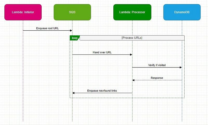
The main components of our serverless crawler are Lambda functions, an SQS queue, and a DynamoDB table. Hereโ€™s a breakdown:

  • Lambda: Two distinct functionsโ€Šโ€”โ€Šone for initiating the crawl and another for the actual processing.
  • SQS: Manages pending crawl tasks as a buffer and task distributor.
  • DynamoDB: Stores visited URLs, ensuring we avoid redundant visits.

Workflow & Logic Rationale:

Initiation:

Starting Point (Root URL):

Logic: The crawl starts with a root URL, e.g., โ€œwww.shanoj.com”.

Rationale: A defined beginning allows the crawler to commence in a guided manner.

Uniqueness with UUID:

Logic: A unique run ID is generated for every crawl to ensure distinction.

Rationale: These guards against potential data overlap in the case of concurrent crawls.

Avoiding Redundant Visits:

Logic: The root URL is pre-emptively marked as โ€œvisitedโ€.

Rationale: This step is integral to maximizing efficiency by sidestepping repeated processing.

The URL then finds its way to SQS, awaiting crawling.

Processing:

Link Extraction:

Logic: A secondary Lambda function polls SQS for URLs. Once a URL is retrieved, the associated webpage is fetched. All the links are identified and extracted within this webpage for further processing.

Rationale: Extracting all navigable paths from our current location is pivotal to web exploration.

Depth-First Exploration Strategy:

Logic: Extracted links undergo a check against DynamoDB. If previously unvisited, theyโ€™re designated as such in the database and enqueued back into SQS.

Rationale: This approach delves deep into one linkโ€™s pathways before backtracking, optimizing resource utilization.

Special Considerations:

A challenge for web crawlers is the potential for link loops, which can usher in infinite cycles. By verifying the โ€œvisitedโ€ status of URLs in DynamoDB, we proactively truncate these cycles.

Back-of-the-Envelope Estimation for Web Crawling:

1. Data Download:

  • Webpages per month: 1 billion
  • The average size of a webpage: 500 KB

Total data downloaded per month:

1,000,000,000 (webpages) ร— 500 KB = 500,000,000,000 KB

or 500 TB (terabytes) of data every month.

2. Lambda Execution:

Assuming that the Lambda function needs to be invoked for each webpage to process and extract links:

  • Number of Lambda executions per month: 1 billion

(One would need to further consider the execution time for each Lambda function and the associated costs)

3. DynamoDBย Storage:

Letโ€™s assume that for each webpage, we store only the URL and some metadata which might, on average, be 1 KB:

  • Total storage needed for DynamoDB per month:
  • 1,000,000,000 (webpages) ร— 1 KB = 1,000,000,000 KB
  • or 1 TB of data storage every month.

(However, if youโ€™re marking URLs as โ€œvisitedโ€ and removing them post the crawl, then the storage might be significantly less on a persistent basis.)

4. SQS Messages:

Each webpage URL to be crawled would be a message in SQS:

  • Number of SQS messages per month: 1 billion

The system wouldย require:

  • 500 TB of data storage and transfer capacity for the actual web pages each month.
  • One billion Lambda function executions monthly for processing.
  • About 1 TB of storage in DynamoDB might vary based on retention and removal strategies.
  • One billion SQS messages to manage the crawl queue.

Stackademic

Thank you for reading until the end. Before you go:

  • Please consider clapping and following the writer! ๐Ÿ‘
  • Follow us on Twitter(X), LinkedIn, and YouTube.
  • Visit Stackademic.com to find out more about how we are democratizing free programming education around the world.

AWS-Based URL Shortener: Design, Logic, and Scalability

Hereโ€™s a behind-the-scenes look at creating a URL-shortening service using Amazon Web Services (AWS).

Users and System Interaction:

  • User Requests: Users submit a long web address wanting a shorter version, or they might want to use a short link to reach the original website or remove a short link.
  • API Gateway: This is AWSโ€™s reception. It directs user requests to the right service inside AWS.
  • Lambda Functions: These are the workers. They perform tasks like making a link shorter, retrieving the original from a short link, or deleting a short link.
  • DynamoDB: This is the storage room. All the long and short web addresses are stored here.
  • ElastiCache: Before heading to DynamoDB, the system checks here first when users access a short link. Itโ€™s faster.
  • VPC & Subnets: This is the AWS structure. The welcoming part (API Gateway) is public, while sensitive data (DynamoDB) is kept private and secure.

Making Links Shorter for Users:

  • Sequential Counting: Every web link gets a unique number. To keep it short, that number is converted into a combination of letters and numbers.
  • Hashing: The system also shortens the long web address into a fixed-length string. This method may produce similar results for different links, but the system manages and differentiates them efficiently.

Sequential Counting: This takes a long URL as input and uses a unique counter value from the database to generate a short URL.

For instance, the URL https://example.com/very-long-url might be shortened to https://short.url/1234AB using a unique number from the database, then converting this number into a mix of letters and numbers.

Hashing: This involves taking a long URL and converting it to a fixed-size string of characters using a hashing algorithm. So, https://example.com/very-long-url could become https://short.url/h5Gk9.

The rationale for Combining:

  1. Enhanced Uniqueness & Collision Handling: Sequential counting ensures uniqueness, and in the unlikely event of a hashing collision, the sequential identifier can be used as a fallback or combined with the hash.
  2. Balancing Predictability & Compactness: Hashing gives compact URLs, and by adding a sequential component, we reduce predictability.
  3. Scalability & Performance: Sequential lookups are faster. If the hash table grows large, the performance could degrade due to hash collisions. Combining with sequential IDs ensures fast retrievals.

Lambda Function for Shortening (PUTย Request)

  1. Input: Long URL e.g. โ€œhttps://www.example.com/very-long-url
  2. URL Exists: Retrieved Shortened URL e.g. โ€œabcd12โ€
  3. Hash URL: Output e.g. โ€œa1b2c3โ€
  4. Assign Number: Unique Sequential Number e.g. โ€œ456โ€
  5. Combine Hash & Number: e.g. โ€œa1b2c3456โ€
  6. Store in DynamoDB: {โ€œhttps://www.example.com/very-long-url“: โ€œa1b2c3456โ€}
  7. Update ElastiCache: {โ€œa1b2c3456โ€: โ€œhttps://www.example.com/very-long-url”}
  8. Return to API Gateway: Shortened URL e.g. โ€œa1b2c3456โ€

Lambda Function for Redirecting (GETย Request)

  • Input: The user provides a short URL like โ€œa1b2c3456โ€.
  • Check-in ElastiCache: System looks up the short URL in ElastiCache.
  • Cache Hit: If the Long URL is found in the cache, the system retrieves it directly.
  • Cache Miss: If not in the cache, the system searches in DynamoDB.
  • Check-in DynamoDB: Searches the DynamoDB for the corresponding Long URL.
  • URL Found: The Long URL matching the given short URL is found, e.g. โ€œhttps://www.example.com/very-long-url“.
  • Update ElastiCache: System updates the cache with {โ€œa1b2c3456โ€: โ€œhttps://www.example.com/very-long-url”}.
  • Return to API Gateway: The system redirects users to the original Long URL.

Lambda Function for Deleting (DELETEย Request)

  • Input: The user provides a short URL they want to delete.
  • Check-in DynamoDB: System looks up the short URL in DynamoDB.
  • URL Found: If the URL mapping for the short URL is found, it proceeds to deletion.
  • Delete from DynamoDB: The system deletes the URL mapping from DynamoDB.
  • Clear from ElastiCache: The System also clears the URL mapping from the cache to ensure that the short URL no longer redirects users.
  • Return Confirmation to API Gateway: After the deletion is successful, a confirmation is sent to the API Gateway, confirming the user about the deletion.

Simple Math Behind Our URL Shortening (Envelope Estimation):

When we use a 6-character mix of letters (both small and capital) and numbers for our short URLs, we have about 56.8 billion different combinations. If users create 100 million short links every day, we can keep making unique links for over 500 days without repeating them.

In Plainย English

Thank you for being a part of our community! Before you go: